Atlanta Crime Data 2009-2019


In [ ]:
 

Research / Resources


Definitions

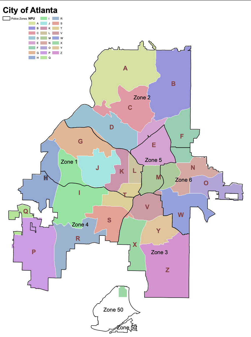
  • 'Beat' - "The City of Atlanta is divided into six unique geographic areas – known as Zones – for the purposes of allocating APD resources. Each Zone is then divided into 13-14 “beats” assigned to a specific officer for patrol purposes.".

  • 'UCR' - Uniform Crime Reporting Number. This number classifies a crime using a number system. Links to chart attached.

  • 'IBR' - Allows for more specific crime types.

  • 'NPU' - "The City of Atlanta is divided into twenty-five (25) Neighborhood Planning Units (NPUs), which are citizen advisory councils that make recommendations to the Mayor and City Council on zoning, land use, and other planning-related matters. ".

Research
Atlanta Police Beat and Zones
NIBRS
UCR CLASSIFICATION ABBREVIATIONS
Atlanta Police Department Crime Data Downloads
Uniform Crime Reporting Handbook

Zones / NPU


Imports


In [38]:
import numpy as np
import matplotlib.pyplot as plt
import pandas as pd
import seaborn as sns
from scipy import stats
import plotly.express as px
from datetime import datetime
from geopy.geocoders import Nominatim
import geopy as gp

Data


In [39]:
atlanta = pd.read_csv("COBRA-2009-2019 (Updated 1_9_2020)/COBRA-2009-2019.csv")
atlanta.head()
/Users/aleia/Library/Python/3.7/lib/python/site-packages/IPython/core/interactiveshell.py:3063: DtypeWarning:

Columns (3,11) have mixed types.Specify dtype option on import or set low_memory=False.

Out[39]:
Report Number Report Date Occur Date Occur Time Possible Date Possible Time Beat Apartment Office Prefix Apartment Number Location Shift Occurence Location Type UCR Literal UCR # IBR Code Neighborhood NPU Latitude Longitude
0 90010930 2009-01-01 2009-01-01 1145 2009-01-01 1148.0 411.0 NaN NaN 2841 GREENBRIAR PKWY Day Watch 8 LARCENY-NON VEHICLE 630 2303 Greenbriar R 33.68845 -84.49328
1 90011083 2009-01-01 2009-01-01 1330 2009-01-01 1330.0 511.0 NaN NaN 12 BROAD ST SW Day Watch 9 LARCENY-NON VEHICLE 630 2303 Downtown M 33.75320 -84.39201
2 90011208 2009-01-01 2009-01-01 1500 2009-01-01 1520.0 407.0 NaN NaN 3500 MARTIN L KING JR DR SW Unknown 8 LARCENY-NON VEHICLE 630 2303 Adamsville H 33.75735 -84.50282
3 90011218 2009-01-01 2009-01-01 1450 2009-01-01 1510.0 210.0 NaN NaN 3393 PEACHTREE RD NE Evening Watch 8 LARCENY-NON VEHICLE 630 2303 Lenox B 33.84676 -84.36212
4 90011289 2009-01-01 2009-01-01 1600 2009-01-01 1700.0 411.0 NaN NaN 2841 GREENBRIAR PKWY SW Unknown 8 LARCENY-NON VEHICLE 630 2303 Greenbriar R 33.68677 -84.49773

Quick Look


In [40]:
print(atlanta.describe(), '\n\n\n')

atlanta.info()
       Report Number  Possible Time           Beat          UCR #  \
count   3.429140e+05  342895.000000  342890.000000  342914.000000   
mean    1.375665e+08    1310.068065     365.391277     594.856463   
std     3.146330e+07     643.618899     170.580194     111.848817   
min     6.104028e+07       0.000000       0.000000     110.000000   
25%     1.112706e+08     830.000000     209.000000     511.000000   
50%     1.331526e+08    1350.000000     402.000000     640.000000   
75%     1.625932e+08    1830.000000     507.000000     670.000000   
max     2.000724e+08    3015.000000     614.000000     730.000000   

            Latitude      Longitude  
count  342914.000000  342914.000000  
mean       33.757281     -84.407407  
std         0.044930       0.047112  
min        33.637500     -84.550500  
25%        33.730310     -84.432130  
50%        33.756670     -84.396360  
75%        33.781830     -84.373470  
max        33.886130     -84.286410   


<class 'pandas.core.frame.DataFrame'>
RangeIndex: 342914 entries, 0 to 342913
Data columns (total 19 columns):
 #   Column                   Non-Null Count   Dtype  
---  ------                   --------------   -----  
 0   Report Number            342914 non-null  int64  
 1   Report Date              342914 non-null  object 
 2   Occur Date               342914 non-null  object 
 3   Occur Time               342914 non-null  object 
 4   Possible Date            342896 non-null  object 
 5   Possible Time            342895 non-null  float64
 6   Beat                     342890 non-null  float64
 7   Apartment Office Prefix  10094 non-null   object 
 8   Apartment Number         68274 non-null   object 
 9   Location                 342912 non-null  object 
 10  Shift Occurence          342914 non-null  object 
 11  Location Type            333698 non-null  object 
 12  UCR Literal              342914 non-null  object 
 13  UCR #                    342914 non-null  int64  
 14  IBR Code                 342744 non-null  object 
 15  Neighborhood             330551 non-null  object 
 16  NPU                      342775 non-null  object 
 17  Latitude                 342914 non-null  float64
 18  Longitude                342914 non-null  float64
dtypes: float64(4), int64(2), object(13)
memory usage: 49.7+ MB

Cleaning


In [42]:
#DROP COLUMNS
atlanta = atlanta.drop(columns=['Apartment Office Prefix', 'Apartment Number', 'Location', 'Location Type'])

# For converting code to crime group
def codes_to_crimes(value):
    if value > 100 and value < 199:
        return 'Homicide'
    elif value > 200 and value < 299:
        return 'Rape'
    elif value > 300 and value < 399:
        return 'Robbery'
    elif value > 400 and value < 499:
        return 'Assault'
    elif value > 500 and value < 599:
        return 'Burglary'
    elif value > 600 and value < 699:
        return 'Larceny'
    elif value > 700 and value < 799:
        return 'Motor_theft'
    elif value > 800 and value < 899:
        return 'Arson'
atlanta['Crime'] = pd.Series(atlanta['UCR #']).apply(codes_to_crimes).astype('str')


atlanta.head()
Out[42]:
Report Number Report Date Occur Date Occur Time Possible Date Possible Time Beat Shift Occurence UCR Literal UCR # IBR Code Neighborhood NPU Latitude Longitude Crime
0 90010930 2009-01-01 2009-01-01 1145 2009-01-01 1148.0 411.0 Day Watch LARCENY-NON VEHICLE 630 2303 Greenbriar R 33.68845 -84.49328 Larceny
1 90011083 2009-01-01 2009-01-01 1330 2009-01-01 1330.0 511.0 Day Watch LARCENY-NON VEHICLE 630 2303 Downtown M 33.75320 -84.39201 Larceny
2 90011208 2009-01-01 2009-01-01 1500 2009-01-01 1520.0 407.0 Unknown LARCENY-NON VEHICLE 630 2303 Adamsville H 33.75735 -84.50282 Larceny
3 90011218 2009-01-01 2009-01-01 1450 2009-01-01 1510.0 210.0 Evening Watch LARCENY-NON VEHICLE 630 2303 Lenox B 33.84676 -84.36212 Larceny
4 90011289 2009-01-01 2009-01-01 1600 2009-01-01 1700.0 411.0 Unknown LARCENY-NON VEHICLE 630 2303 Greenbriar R 33.68677 -84.49773 Larceny

Sampling


In [43]:
# *****************************
# HIGHLY IMPORTANT while testing
# *****************************

# Sample data
# print("Original Data Stats: \n")
# print(atlanta.describe())

# print('\n--------\n')

# atlanta = atlanta.sample(frac=0.01)  # 1% sample set
# print(atlanta.describe())

Heatmap Correlation


In [44]:
sns.heatmap(atlanta.corr())
Out[44]:
<matplotlib.axes._subplots.AxesSubplot at 0x131e0edd0>

Conclusions


Most can be ignored, but the 'Beat' vs 'UCR #' is interesting. It is not a high correlation but one is there. It does show that there is at least some relation between the Zone of town lived in and the type of crime committed.

Pairplot


In [45]:
sns.pairplot(atlanta)
plt.show()

Conclusions


.....

Pie chart of Crimes


In [52]:
fig = px.pie(atlanta, values='UCR #', names='Crime', title='Crimes in Atlanta', color_discrete_sequence=px.colors.sequential.RdBu)
fig.show()

Conclusions


No arsons or rapes were reported! Not sure if this is due to gaps in the data reporting...

Crime Levels per Neighborhood


In [53]:
fig = px.histogram(atlanta, x="Neighborhood", title='Crime by Neighborhood')
fig.show()

Conclusions


The neighborhoods with the largest crime rates are Midtown, Downtown, and Old Fourth Ward.

Location


In [54]:
BBox = ((atlanta.Longitude.min(), atlanta.Longitude.max(),atlanta.Latitude.min(), atlanta.Latitude.max()))
BBox
Out[54]:
(-84.5505, -84.28641, 33.6375, 33.88613)
In [55]:
img = plt.imread('map.png')
fig, ax = plt.subplots(figsize = (15,12))
ax.scatter(atlanta.Longitude, atlanta.Latitude, zorder=1, alpha= .1,c='b', s=10)
ax.set_title('Plotting Crime Map')
ax.set_xlim(BBox[0],BBox[1])
ax.set_ylim(BBox[2],BBox[3])
ax.imshow(img, zorder=0, extent = BBox, aspect= 'equal')
Out[55]:
<matplotlib.image.AxesImage at 0x1335ac950>

Conclusions


There is more crime the closer to the city you are. Also there seems to be less crime around the airport.

In [ ]: